기록: UCL Course on RL 요약 및 정리 (Lecture 4: Model-Free Prediction)

This post covers not only Lecture 4: Model-Free Prediction (davidsilver.uk) but also:

• Bernoulli trial - Wikipedia
• Geometric distribution - Wikipedia
• Memorylessness - Wikipedia
• The entire course materials can be found on the following page: Teaching - David Silver.

Lecture Goal

• Solve an unknown MDP
• All information of an MDP is not necessarily given (e.g., reward, transition probabilities, etc.)
• Model-free prediction: estimate the value function of an unknown MDP (this lecture)
• Monte-Carlo, Temporal-difference, TD($\lambda$)
• Model-free control: optimize the value function of an unknown MDP (lecture 5)

Monte Carlo | via Forbes Travel Guide

Monte-Carlo Reinforcement Learning

• MC methods learn directly from episodes of experience
• MC is model-free: no knowledge of MDP transitions/rewards
• MC learns from complete episodes: no bootstrapping
• MC uses the simplest possible idea: value = mean return
• Warning: can only apply MC to episodic MDPs
• All episodes must terminate (like Go and Atari games)

Monte-Carlo Policy Evaluation

• Goal: evaluate $v_{\pi }$ from complete episodes of experience under policy $\pi$
• $\pi (a|s)$를 따라 action을 sampling(또는 결정)해가면서 최종적으로 게임이 종료되는 termination state까지 간 다음에 최종 return를 계산한다. 이렇게 한 번의 episode가 끝나고 나면 다시 $S=s$로 돌아가서 action sampling을 해가면서 또 다시 episode를 구성하고 reward를 계산한다. 이렇게 무수히 많은 episode를 경험하여 return의 표본 평균을 구하면, 결국 큰 수의 법칙(law of large numbers)에 의해 $v_{\pi }=\mathbb{E}[G_t|S_t=s]$와 매우 가까워지게 된다.
• $G_t=R_{t+1}+\gamma R_{t+2}+\cdots +{\gamma }^{T-1}{R}_T$

First-Visit Monte-Carlo Policy Evaluation

• To evaluate state $s$, for each episode,
• Note: episode는 agent의 action과 환경의 state transition으로 진행됨
• The first time-step $t$ that state $s$ is visited in an episode,
• Note: 한 episode는 여러 state로 구성되므로, episode 동안 처음 방문하는 모든 state에 대해 아래 $N(s),V(s)$를 update하는 꼴
• Increment the counter $N(s)\leftarrow N(s)+1$
• Increment the value estimator $V(s)\leftarrow V(s)+\frac{1}{N(s)}(G_t-V(s))$
• By law of large numbers, $V(s)\to v_{\pi }(s)$ as $N(s)\to \mathrm{\infty }$
• In non-stationary problems, it can be useful to track a running mean (i.e., forget old episodes) $V(s)\leftarrow V(s)+\alpha (G_t-V(s))$
• $\alpha$가 1에 가까워질수록 현재 $G_t$에 가중치를 두고 0에 가까워질수록 과거의 estimate에 가중치를 둠
• Policy를 고정하고 policy evaluation을 할 때는 해당 policy에 대한 value는 고정되어 있으므로 현재든 과거든 동일한 가중치를 두는 게 상식적이지만, value iteration처럼 policy 자체가 매 iteration마다 바뀌는 경우 (특히 점점 더 policy가 좋아지는 경우), 현재에 가까울 수록 큰 가중치를 두는 게 상식적이다.

Every-Visit Monte-Carlo Policy Evaluation

• To evaluate state $s$
• Every time-step t that state $s$ is visited in an episode,
• Note: 한 episode는 여러 state로 구성되므로, episode 동안 방문하는 모든 state에 대해 아래 $N(s),V(s)$를 update하는 꼴
• Increment the counter $N(s)\leftarrow N(s)+1$
• Increment the value estimator $V(s)\leftarrow V(s)+\frac{1}{N(s)}(G_t-V(s))$
• By law of large numbers, $V(s)\to v_{\pi }(s)$ as $N(s)\to \mathrm{\infty }$

Temporal-Difference Learning (시간차 학습)

• TD methods learn directly from episodes of experience
• Non-episodic game에도 적용될 수 있다. MC와 다른 점.
• TD is model-free: no knowledge of MDP transitions/rewards
• TD learns from incomplete episodes, by bootstrapping
• 몇 번의 state transition을 통해 국소적인 subpath만 구성한 후 value를 추정한다. 따라서 ending이 없는 게임에도 활용할 수 있다.
• Subpath가 구성됐으면 종점 state의 value를 다시 어떤 방법으로 추정한다 (guess). 그 후 subpath 내의 states의 values와 합산하여 subpath 시작점 state의 value를 추정한다 (guess).
• MC는 ending까지 쭉 state transition을 하여 global하고 완전한 path하나씩 추출하여 value를 추정한다.
• TD updates a guess towards a guess.

Temporal-Difference Policy Evaluation

• Goal: learn $v_{\pi }$ online from experience under policy $\pi$
• Incremental every-visit Monte-Carlo
• Update value $V(S_t)$ toward actual return $G_t$ of an episode
• $V(S_t)\leftarrow V(S_t)+\alpha (G_t-V(S_t))$
• Simplest temporal-difference learning algorithm: TD(0)
• Note: 0의 의미가 무엇인지는 나중에 설명
• Fisrt, initialize $V(s)\mathrm{\forall }s$
• Update value $V(S_t)$ toward estimated return $R_{t+1}+\gamma V(S_{t+1})$
• $V(S_t)\leftarrow V(S_t)+\alpha (R_{t+1}+\gamma V(S_{t+1})-V(S_t))$
• $V(S_{t+1})$가 이미 계산돼있다고 가정. 없으면 초기값을 어떤 상수로 준다.

MC vs. TD

• TD can learn before knowing the final outcome
  • TD can learn online after every step
  • MC must wait until the end of an episode before the return is known
• TD can learn without the final outcome
• TD can learn from incomplete sequences
• 그래서 초반엔 잘못된 update가 많다. $V(S_{t+1})$ 자체도 확실치 않으므로. 그래서 $\alpha$를 너무 적게 주면 ($<0.1$) 과거의 추정치에 너무 매몰돼서 결과적으로 bias가 상당히 심해진다. 초반 수렴은 빨라도. 계산이 진행됨에 따라 점진적으로 $\alpha$를 늘려주는 게 좋다.
• Biased estimate
• MC can only learn from complete sequences
• Unbiased estimate
• TD works in continuing (non-terminating) environments
• MC only works for episodic (terminating) environments

Bias/Variance Trade-Off

• MD
• A return $G_t=R_{t+1}+\gamma R_{t+2}+\cdots +{\gamma }^{T-1}{R}_T$ is unbiased estimate of $v_{\pi }(S_t)$
• Since $v_{\pi }(S_t)=\mathbb{E}[G_t]$
• TD
• TD target $R_{t+1}+\gamma V(S_{t+1})$ is biased estimate of $v_{\pi }(S_t)$
• Bias/variance trade-off
• TD target is much lower variance than the return:
• A return depends on many random actions, transitions, rewards
• MC: 매 transition마다 randomness가 추가 되면서 결과가 매우 noisy하게 됨
• TD target depends on one random action, transition, reward
• MC has high variance, zero bias
• Good convergence properties
• (even with function approximation, it just converges to the correct answer)
• Function approximation이란 기법의 사용에 관해서는 나중에 다룰 예정
• 대강 말하자면, 이때까지는 $v_{\pi }(s)$를 추정할 때 각 state를 개별적으로 다뤘다. 그러나 $v_{\pi }(s)$도 state에 관한 함수이므로, 근접한 state들 끼리 어떤 연관성이 있을 수 있다 (see the random walk example on the 19th slide of Lecture 4: Model-Free Prediction (davidsilver.uk)). Function approximation 기법은 state function을 단순한 수의 나열이 아니라 function으로 인식하고 더 지능적으로 state function을 추정하는 방법이다. 예를 들어 state와 value 간의 linear regression 성향이 있는 것으로 관측된다면 그런 추측을 통해 $v_{\pi }(s)$를 더 잘 추정할 수 있다.
• Not very sensitive to the initial value function
• Very simple to understand and use
• TD has low variance, some bias
• Usually more efficient than MC
• TD(0) converges to $v_{\pi }(s)$
• (but not always with function approximation)
• More sensitive to the initial value function
• MC vs. TD bias/variance trade-off visualization
  
  



• Idea: 초반엔 알파 낮은 TD로 학습하다가 점진적으로 알파를 늘려나가고, 일정 에러를 달성하면 그 뒤부터는 unbiased한 MC estimate를 쓰면 어떨까?
• 비슷한 아이디어를 적용한 논문이 2019년도 제안됨: Adaptive Temporal-Difference Learning for Policy Evaluation with Per-State Uncertainty Estimates (neurips.cc)

MC vs. TD (2)

• TD exploits Markov property
• TD는 한 state에서 subpath를 만들기 위해 다른 state의 (estimated) value를 참고함. 이것 자체가 chain의 성질을 활용하는 것. 또한 후속 state의 value를 더하는 식 자체가 Markov property에 의해 유도되는 것.
• Episode를 더 많이 참고할 수록 state $s$의 후속 state $s^{\prime }$의 value가 정확해지고, 이는 $V(s)$의 오차도 줄인다. 모든 state의 정확성은 상호 의존한다.
• Usually more efficient in Markov environments
• MC does not exploit Markov property
• MC의 경우 value estimation system이 관찰하는 것은 오직 한 state에서 시작한 episode가 끝날 때 받는 최종 reward (intermediate states의 value를 더하는 과정은 굳이 system이 알 필요 없음). 그것을 평균내는 것 뿐.
• 후속 state의 value estimation이 얼마나 정확한지는 현재 state와 무관하다.
• Usually more effective in non-Markov environments
• Note: MDP를 구성하기 위해서는 state가 Markov여야 한다. 그러나 로봇의 센서 정보로 state를 구성한다고 할 때 마구잡이로 구성하면 state가 Markov가 아닐 수 있다. 이런 경우에는 TD를 사용하면 제대로 된 해를 찾지 못할 수 있다. MC는 여전히 잘 동작한다.
• Note: 이는 강의 노트의 Batch MC and TD 예시에서 잘 드러난다.

DP vs. MC vs. TD

• Dynamic programming backup

• DP는 한 state에서 전이할 수 있는 모든 state를 고려한다.
• 또한 $\pi (a|s),T$를 이미 알고있으므로 직접 기대값을 구할 수 있다.
• ${\mathbb{E}}_{X\sim \mathrm{P}(X)}[X]=\sum _{i=1}{x}_i\mathrm{P}(x_i)$
• 미리 구해둔 (또는 초기값) 바로 다음 state $S_{t+1}$의 value들과 Bellman expectation equation을 통해 현재 state의 value를 정확히 계산할 수 있다. (다만, policy evaluation의 iteration 중에는 각 state의 정확한 value를 구할 수 없으므로 David Silver는 estimate라고 표현한다.)
  
  
• Temporal-difference backup

• TD와 MC는 $T$를 모르는 unknown MDP 문제를 푸는 게 목적이다.
• 환경이 agent에게 state(와 reward)를 알려주면 agent는 그의 정책 $\pi (a|s)$을 통해 action을 sampling한다.
• 그 뒤, action을 환경에게 알려주면 환경은 그의 $T$를 통해 다음 state를 agent에게 알려준다. 이때 환경은 확률분포 $T$를 알고 있으므로 $T(s^{\prime }|s,a)$ 값을 계산(evaluation)할 수 있지만, agent는 계산할 수 없다. 즉, unknown MDP.
• 미리 구해둔 (또는 초기값) $s^{\prime }$의 value estimate과 Bellman expectation equation을 통해 $V(s)$를 추정할 수 있다.
  
  
• Monte-Carlo backup

• TD(0)와 비슷하지만, action sampling을 recursive하게 반복하다가 최종적으로 termination state를 만나서 episode가 종료하고 난 뒤, 그 complete path의 reward $G_t$를 구한다.
• 미리 구해둔 value를 활용하지 않는다.

Bootstrapping and Sampling

• Sampling: a value update samples a (sub-)path to estimate the expectation
• DP does not sample (직접 기대값을 구할 수 있음)
• TD samples a subpath
• MC samples a path
• Bootstrapping: a value update exploit the previous value estimation (미리 구해둔 value를 활용)
• DP bootstraps
• TD bootstraps
• MC does not bootstrap

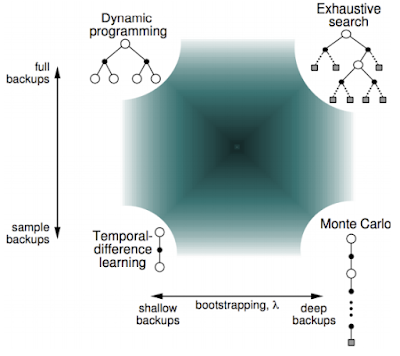
Unified View of RL

TD($\lambda$)

• $n$-step prediction
• TD(0)에서는 한 step만 lookahead하여 value를 추정하였다. 그러나 subpath의 길이가 꼭 1일 필요는 없을 것이다:

• $n$-step return
• $G_t^{(n)}:=R_{t+1}+\gamma R_{t+2}+{\gamma }^2{R}_{t+3}+\cdots +{\gamma }^{n-1}{R}_{t+n}+{\gamma }^{n}V(S_{t+n})$
• $n\to \mathrm{\infty }$ 이면 MC가 된다.
• $n$-step TD
• $V(S_t)\leftarrow V(S_t)+\alpha (G_t^{(n)}-V(S_t))$
• TD($\lambda$) (forward-view)
• 몇 step을 쓰는 게 가장 좋을까? 실제로 MDP의 크기나 문제 세팅에 따라 최적의 step수는 계속 달라진다. 더 robust한 알고리즘을 만들기 위해 여러 step의 TD를 섞어서 쓸 수 없을까? 이런 고민으로 제안된 게 TD($\lambda$)이다. TD($\lambda$)는 가능한 모든 길이의 subpath를 고려한다.
• $\lambda$-return
• $G_t^{\lambda }=(1-\lambda )\sum _{n=1}^{\mathrm{\infty }}{\lambda }^{n-1}{G}_t^{(n)}$
• $V(S_t)\leftarrow V(S_t)+\alpha (G_t^{\lambda }-V(S_t))$
• Note: $\lambda =0$이면 길이 1의 subpath만 고려한다(현재 state와 바로 다음 state). $\lambda \to 1$일수록 다양한 길이의 subpaths를 고려한다. 
• Note: $G_t^{\lambda }$의 의미 해석: 짧게 말해 geometric distribution. 매 state에서 $1-\lambda$의 확률로 terminate하고, $\lambda$의 확률로 transition 한다고 하자. 이렇게 $n$을 정할 때의 기대 reward가 $G_t^{\lambda }$이다.
• 1-step backup할 확률: $1-\lambda$
• 2-step backup할 확률: $\lambda (1-\lambda )$
• $⋮$
• n-step backup할 확률: ${\lambda }^{n-1}(1-\lambda )$
• Note: The geometric distribution is the only memoryless discrete distribution. 그래서 TD(0)나 TD($\lambda$)나 똑같은 memory efficiency를 지닌다.
• Note: TD(0)는 one-step bootstrap을 하기 때문에 후속 state의 value가 update 되더라도 step이 멀리 떨어져 있으면 반영이 바로 안되고 episode를 여러 번 돌려야 반영된다. TD($\lambda$)는 $\lambda$를 조정하여 얼마나 한 state의 변화가 이전 state들에 반영될지 결정한다:

• TD($\lambda$)는 꽤 robust한 알고리즘이며, 대충 $\lambda =0.9$를 쓰면 최적이라고 한다.
• Vanilla TD(0)나 MC와는 다르게, bias/variance 간의 균형을 잘 잡아준다.
• TD($\lambda$) (backward-view)
• 다만 forward-view의 문제점은 단번에 $G_t^{\lambda }$를 구하기 위해서 결국 MC처럼 episode의 끝을 봐야한다는 점이다.
• Backward-view TD updates value estimates online, at every step, from incomplete sequences. 또한 동시에 모든 state의 value를 update한다.
• Def. Eligibility Traces
• $\mathrm{\forall }s\in S,t\in [0,\mathrm{\infty }),$ define eligibility traces $E_t(s)$ as follow:
• $$\begin{gathered} E_0(s)=0, \\ {E}_t(s)=\gamma \lambda E_{t-1}(s)+\mathbf{1}(S_t=s) \end{gathered}$$
• 따라서 state $s$에 잦게 방문할 수록 eligibility trace는 커지고, 어떤 시점에 방문을 한 뒤부터 방문을 더 안하고 있으면 지수적으로 줄어든다.
• Backward-view TD($\lambda$)
• Keep an eligibility trace for every state
• Update value $V(s)$ for every state
• In proportion to eligibility traces:
• $$\begin{gathered} {\delta }_t=R_{t+1}+\gamma V(S_{t+1})-V(S_t) \\ V(s)\leftarrow V(s)+\alpha {\delta }_t{E}_t(s) \end{gathered}$$
• $E_t(s)$의 정의에 따라 어느 한 시점에 방문을 하면 그 뒤부터 지수적으로 ${\delta }_t$에 적용되는 가중치가 줄어든다.
• Thm. Forward-backward Equivalence
• Offline updates: updates are accumulated within an episode but applied in batch at the end of an episode.
• The sum of offline updates is identical for forward-view and backward-view TD($\lambda$):
• $\underset{T\to \mathrm{\infty }}{lim}\sum _{t=1}^T\alpha {\delta }_t{E}_t(s)=\underset{T\to \mathrm{\infty }}{lim}\sum _{t=1}^T\alpha (G_t^{\lambda }-V(S_t))\mathbf{1}(S_t=s)$
• Note: online update를 사용하면 eligibility trace term을 살짝 바꿈으로써 forward-view와 backward-view를 동치로 만들 수 있다.
• Sketch of Proof)
• 모든 항을 비교하긴 귀찮으니 양변의 항 ${\lambda }^{l-1}\mathbf{1}(S_t=s)$의 계수를 비교해서 같은지 비교하면 된다.
• Eligibility trace의 recursive한 정의를 풀면(unroll):
• $E_t(s)=(\gamma \delta {)}^0\mathbf{1}(S_t=s)+(\gamma \delta {)}^1\mathbf{1}(S_{t-1}=s)+\cdots +(\gamma \delta {)}^{t-1}\mathbf{1}(S_1=s)$