기록: UCL Course on RL 요약 및 정리 (Lecture 8: Integrating Learning and Planning)
This post covers Lecture 8: Integrating Learning and Planning (davidsilver.uk):
- The entire course materials can be found on the following page: Teaching - David Silver.
Lecture Goal
- Opening remarks:
- 지금껏 known MDP의 경우, model을 알고 있으므로 dynamic programming등 planning 기법을 이용하여 최적의 value function이나 policy를 구할 수 있었다 (이를 MDP를 푼다고 표현한다).
- 지금껏 unknown MDP의 경우, environment와의 상호작용(experience)을 통해 최적의 value/policy를 학습하였다 (learning).
- Unknown MDP를 풀 때도 experience를 통해, policy나 value만 학습하는 게 아니라, model (i.e., expected rewards and transition probability) 자체를 학습한다면 planning 기법을 사용하여 좀 더 효율적으로 MDP를 풀 수 있지 않을까?
- 본 강의에서는 unknown MDP를 풀기 위해 learning과 planning을 통합적으로 이용하는 model-based reinforcement learning 방법을 배운다.
- Learning, simulation & planning, Dyna-Q, Monte-Carlo tree search

Model
- Given an MDP \((S,A,T,R)\), a model \(M=(T,R)\) represents state transitions and expected rewards:
- \(S_{t+1} \sim T(S_{t+1}|S_t,A_t)\)
\(R_{t+1} = R(S_t,A_t)\) - Note: model은 환경 그 자체가 아니다. 환경에서 MDP를 최적화할 때 가장 핵심 요소들만 뽑아 구성한 것이라고 보면 된다. 예를 들어, 실제로 immediate reward는 random variable이지만 model은 expectation만 알면 되므로 scalar인 expected reward만 포함한다.
Value vs. Model
- 일반적으로 value function은 state에 대한 (e.g., Chess에서 각 장기말의 현재 위치) 변화가 크다.
- 학습하기 어렵고 approximator를 쓸 때도 문제가 있다. Linear model은 smooth하기 때문에 pluctuation이 심한 value function을 제대로 근사하지 못할 수도 있다.
- 또한 한 state의 value는 해당 state의 reward에만 관련있는 게 아니라, Bellman expectation equation에 따라 여러 state의 reward와 큰 연관이 있고, 어떤 transition path를 취하냐에 따라서 return의 noise도 매우 심하다.
- 그러나 model은 environment를 더 compact하게 해석할 수 있도록 정보를 제공한다.
- 예를 들어, Chess에서 model은 Chess의 승리 조건(reward)과 움직이는 규칙(action을 취한대로 deterministic하게 결정) 뿐이다.
- 또한, 한 state의 reward와 transition은 오직 그 state에서의 경험에만 의존하므로 학습하기가 상대적으로 쉽다.
- 따라서 model은 value보다 학습하기 더 쉽고, model을 알 경우 DP나 tree search (곧 배울 Monte Carlo tree search 등) 등 planning을 통해 좋은 정책을 세울 수 있다.
Model-Free and Model-Based RL
- Model-free RL
- No model
- Learn value function (or policy) from experience
- Model-based RL
- Learn a model from experience
- Plan value function (or policy) from model

- Assumptions:
- State space and action space are known
- 상태의 종류, 액션의 종류에는 뭐가 있는지 정도는 알아야 함
- Typically assume conditional independence between state transitions and rewards.
- \(\mathbb{P}[S_{t+1},R_{t+1}|S_t,A_t] = \mathbb{P}[S_{t+1}|S_t,A_t]\mathbb{P}[R_{t+1}|S_t,A_t] \)
- Pros
- Can efficiently learn model by supervised learning methods
- Any supervised learning method can be used.
- Can reason about model uncertainty
- 경험을 적게 해본 experience와 많이 해본 experience는 같은 expected reward라도 다르게 취급해야 할 수 있다. 이를 위한 것이 Bayesian model-based reinforcement learning
- CS885 Lecture 10: Bayesian RL - YouTube
- Bayesian Reinforcement Learning: A Survey
- 실제로 풀려는 문제가 정확히 MDP인 건 아닐 때, model learning을 통해 대충 근사할 수 있다.
- Cons
- Two sources of the approximation error
- Learn a model first, then construct a value function
Model Learning
- Estimate the model from experiences (or episodes)
- Episode \(= \{S_1, A_1, R_2, \cdots, S_T\}\)
- Estimator \(M_{\eta} \approx M\)
- This is nothing but a supervised learning problem
- \(S_1, A_1 \rightarrow R_2, S_2 \\
S_2, A_2 \rightarrow R_3, S_3 \\
\vdots \\
S_{T-1}, A_{T-1} \rightarrow R_T, S_T \) - Learning \(s,a \rightarrow r\) is a regression problem
- Learning \(s,a \rightarrow s'\) is a density estimation problem
- Pick loss functions (e.g., mean-squared error, KL divergence, etc.)
- Find parameters \(\eta\) that minimize empirical loss
- Model을 학습(learning)하여 simulation and planning으로 MDP를 풀어내는 기법
- Learning
- DQN (Lecture 6) 등에서 활용한 experience replay는 (one-step) experience를 (state, action, reward의 순열) 단순히 array 등의 형태로 저장공간(replay buffer)에 보관해둔 다음 minibatch를 구성할 때 저장공간에서 필요한 만큼 뽑아서 쓰는 기법
- Model learning은, experience replay처럼 단순히 replay buffer를 쓰는 대신에, data-driven하게 experiences로 부터 environment 작동 원리를 파악하는 것
- \((s,a,s',r)\)을 단순히 암기하는 것과, \(s,a \rightarrow s', r\)의 규칙(전이 확률)을 학습하는 것의 차이
- Note: learning은 실제 환경과 상호작용을 통해 이루어지므로, 로봇을 움직여서 정보를 얻는 것처럼, 비용이 상대적으로 많이 든다.
- Simulation
- Model learning을 한단 건 결국 transition probabilities와 rewards를 예상할 수 있단 것
- 이를 이용하여 환경과의 직접적인 상호작용 없이 임의로 experience를 생성
- Machine learning에서 자주 활용하는 data augmentation과 비슷한 역할
- Experience replay와 batch sampling이 DQN의 학습 안정화에 큰 역할을 하는 것처럼, simulation을 통해 임의로 experiences를 찍어낼 (augmentation) 수 있다면 학습이 자명하게 안정됨
- Overshoot이긴 하지만 generative model, variational model을 끼얹는 것도 재밌을 듯
- Note: simulation은 기존 학습한 model을 통해 컴퓨터 레벨에서 experience를 만들어 내는 것이므로, 비용이 상대적으로 적게 든다.
- Planning
- (Model learning을 통해 구한) transition probabilities와 rewards를 알면 Bellman expectation and maximization equations으로 MDP를 풀 수 있음
- Value iteration
- Policy iteration
- Dynamic programming
- Monte Carlo tree search (this lecture)
- Minimax tree search (last lecture)
- \(\vdots\)
- 이미 모든 정보를 다 아는 (또는 추정한) 상태에서 최적의 경로나 policy를 계획하는 것
Examples of Models (Model Estimators)
- 이제부터 본 강의에서 model은 model estimator이다.
- Table lookup model
- Linear expectation model
- Linear Gaussian model
- Gaussian process model
- Deep Belief Network model
Learning: Table Lookup Model
- \(s,a \rightarrow s', r\)을 학습하기 위해, hashmap등을 이용해서 cumulative reward at \((s,a)\), \(N(s,a), N(s,a,s')\)을 매 transition마다 저장 및 업데이트한다. 그러면:
- \(R(s,a) = \mathbb{E}[R_{t+1}|S_t=s,A_t=a] \approx (\mathrm{cumulative\; reward})/N(s,a) \\
T(s'|s,a) = \mathbb{P}[S_{t+1}=s'|S_t=s, A_t=a] \approx N(s,a,s')/N(s,a)\) 
- 오른쪽은 experience, 왼쪽은 table lookup을 사용해 만든 estimated MDP를 시각화한 것
Simulation
- Model을 학습하여 예측한 transition probabilities와 rewards를 이용해 experience를 무작위로 생성할 수 있음
- State \(s\)에서 random하게 action \(a\)를 고른 다음,
- Table lookup 등으로 \(T(s'|s,a)\)를 모든 \(s' \in S\)에 관해 구한다. 이때 기본 가정에 의해 \(S\)에 어떤 element \(s\)가 있는지는 알 수 있으므로 for-loop 등을 돌 수 있다.
- State transition에 관한 probability mass function을 구해서 그에 맞춰 sampling하여 다음 상태 \(s'\)를 뽑는다. Reward도 table에서 계산한다.
- 이 과정을 반복하여 experience를 생성한다.
Simulation-Based Planning (Sample-Based Planning)
- 사실 table lookup model등 model만 세워도 transition probabilities와 rewards를 추정하여 Bellman equations (matrix form)을 푸는 것 만으로 MDPs의 최적 policy/value를 구할 수 있다.
- 그러나 보통은 아래와 같은 simulation-based planning (iterative methods)가 더 시간 효율적이다.
- Simulation-based planning
- Use the model only to generate samples
- Sample experiences from model
- Apply model-free RL to samples, e.g.:
- MC/TD control
- Sarsa
- Q-learning
Integrating Learning and Planning
- 당연하게도, model은 환경과 상호작용을 통한 experiences로 배우기 때문에 experiences 수가 너무 적거나 하는 이유로 (estimated) model 자체가 실제 model과 너무 차이가 많으면 estimated model을 기반으로 planning하는 model-based RL의 성능은 나빠진다.
- 따라서 learning, planning, real experience 모두 통합적으로 사용해야 한다.
- 이번 챕터를 통해 two sources of experience를 배웠다:
- Real experience (sampled from true MDP)
- Simulated experience (sampled from estimated MDP)
- RL revisited
- Model-free RL
- No model
- Learn value/policy from real experience
- Model-based RL
- Learn a model from real experience
- Plan value/policy from simulated experience
- Data augmentation을 통해 학습 안정화
- Dyna
- Learn a model from real experience
- Learn and plan value/policy from real and simulated experience
Dyna-Q Algorithm

- Model-based Q-learning이라고 보면 된다 (off-policy).
- 참고로 Q-learning 알고리즘은 다음과 같다:

- Dyna-Q는 real experience를 value update에 한 번만 사용하고 버리거나, DQN처럼 단순히 replay buffer에 저장하는 게 아니라, \((r,s')\)를 생성해낼 수 있는 모델을 real experience로 학습시킨다.
- 그런 다음, 모델을 이용해 (현재 상태와 다음 상태에 관한) simulated experience를 생성해낸 뒤 다시 value를 update해서 기존 real experience에서 습득한 과거의 지식을 계속 value가 상기하도록 한다 (calibration).
- 따라서 과거의 경험을 매우 잘 활용할 수 있다. 사골처럼.
- 또한, 바로 다음 action을 덥썩 덥썩 취하는 게 아니라 agent 스스로 과거의 경험을 반추하는 시뮬레이션을 통해 액션을 결정하므로써 action 하나 하나의 파급력과 리스크가 큰 문제를 풀 때 유용하다.

- 결론은, 더 발전된 Dyna-Q+나 Dyna-2 사용하는 게 좋다.
- Exploration을 잘해서 중간에 환경이 바뀌어도 RL 잘 수행 (방문하지 않은 state에 방문하는 것을 장려함)

Simulation-Based Search
- Opening comment: Dyna-Q 등 지금껏 배운 model-based RL은, 전체 MDP를 모사하기 위해 model을 학습하였고, 이를 통해 experience를 인공적으로 만들어내면서 value function을 update하였다. 그러나 현재 상태에서 당장의 액션을 잘 취하기 위해 learned model을 사용할 방법은 없을까? Simulation-based search가 한 가지 해법을 제공한다.
- Simulation-based search:
- 학습한 model을 이용해 episode sampling을 (simulation) 하면서,
- 현재 state를 root로 하는 tree를 만들어
- 미래 state들의 value를 (implicit/explicit하게) 저장 및 업데이트하고,
- 최종적으로는 가장 value가 높은 action을 찾는 (search) 방법론
- Dyna-Q는 one-step experience만 sampling 하지만, simulation-based search는 (예를 들어 Monte-Carlo evaluation을 쓴다면) termination state까지 쭉 simulation을 하여 full episode 전체를 샘플링한다.
- Note: search 자체는 RL이 아니다. RL 알고리즘 내부의 state update 단계를 위해서 쓰는 것.
- Forward search

- Simulation-based search

- Apply model-free RL to simulated episodes
- Monte-Carlo control을 사용하면 Monte-Carlo search
- Sarsa를 사용하면 TD search
- Simple Monte-Carlo search
- Goal: current state \(S_t = s\)의 각 action의 value를 추정하여 어떤 action을 취하는 게 가장 좋을지 판단 (max search)
- Assumption: 학습한 model은 있고, simulation 중 사용할 policy도 있음 (random policy 등)
- For each action \(a \in A\) at \(s_t\),
- Simulate multiple episodes (\(K\)-times) from current state \(s_t\) and action under given model simulation policy \(\pi\)
- \(\left\{s_t,a,R^{k}_{t+1},S^{k}_{t+1},A^{k}_{t+1},\cdots,S^{k}_{T}\right\}^{K}_{k=1}\sim M_{\eta},\pi\)
- 각 episode에서 얻은 결과 (return) 취합 (Monte-Carlo evaluation)
- \(Q(s_t, a) = \frac{1}{K}\sum_{k=1}^{K}G_t\)
- 이는 \(q_{\pi}(s_t,a)\)로 수렴
- \(Q(s_t,a)\) 최댓값을 주는 액션 하나를 택한다.
- Note: learned model이 아니라 실제 환경과 상호작용을 통해 최댓값을 찾아내려 한다면 매 episode 마다 state \(s_t\)로 실제 물리적으로 되돌아가야 한다 (예: 로봇 옮기기). Model learning을 통해 이런 번거로운 과정을 줄일 수 있다. 이게 기존 Monte-Carlo value iteration 과의 실질적인 차이점이다. 실제 물리 공간에서 환경과 상호작용하는 게 컴퓨터로 시뮬레이션하는 것 만큼 매우 빠르고 위험요소도 없다면 (교통사고 등) 굳이 모델을 학습하고 시뮬레이션할 필요가 없을지도.
Monte-Carlo Tree Search
- Opening comment: 굳이 simple MC search에서 complete episode를 sampling 해놓고 시작 state의 action-value만을 추정하고 episode 중간에 선택한 수많은 action에 관한 정보는 다 날려버릴 필요가 있을까? 중간에 방문한 state와 action에 관한 정보도 search 과정에서 tree에 저장해두면 좀 더 efficient하게 search할 수 있을 것이다 (즉, simulation policy \(\pi\)를 개선).
- MCTS: episode sampling하면서 episode 내의 \((s, a)\)에 관한 정보도 (action-value) 저장해두자. Simulation policy \(\pi\)도 가만히두지 말고 점진적으로 개선하자. MCTS를 이용하면 주어진 model에 관해 최적의 \(q_{*}(s_t,a)\)에 수렴하는 \(Q(s_t,a)\)를 구하여 action 선택에 사용할 수 있다.
- Algorithm
- AlphaGo의 알고리즘과 모델
- Note: 실제 AlphaGo 알고리즘은 MCTS와 단순한 RL보다 더 복잡한 구성 요소들이 많다. 여기서는 간략하게 나마 RL 분야에서 MCTS와 simulation-based forward search의 이점만 이해하고 넘어가자.
- 위 알고리즘은 다음처럼 evaluation과 simulation 부분으로 나눠서 생각할 수 있다.
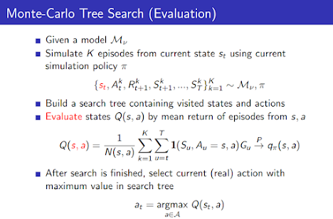

- 이렇게 현재 state에서 모든 action에 대한 \(Q(s_t,a)\)를 구한 뒤 Monte-Carlo control을 통해 최종 action 선택 (global policy improvement)
- Pros
- A highly selective best-first search
- Uses sampling to break the curse of dimensionality
- 굳이 모든 state-/action-space 탐험할 필요가 없고, sampling을 하면서 얻어걸린 space(와 \(\epsilon\)-greedy로 무작위로 선택된 space)만 탐험하면 됨
- Computationally efficient, anytime, parallelizable
- Anytime: an anytime algorithm is an algorithm that can return a valid solution to a problem even if it is interrupted before it ends (즉, 알고리즘을 언제든지 종료해도 최적은 아니지만 그래도 쓸만한 유효한 해를 뱉어냄).
- Other great materials
TD Search
- Using TD instead of MC (bootstrapping)
- TD search applies SARSA control to sub-MDP from the current state
- MC tree search applies MC control
- MC vs. TD
- TD learning reduces variance but increases bias
- TD learning is usually more efficient than MC
- TD(\(\lambda\)) can be much more efficient than MC
- TD search

Dyna-2
- Long-term memory is updated from real experience
- Short-term memory is updated from simulated experience


댓글
댓글 쓰기