기록: UCL Course on RL 요약 및 정리 (Lecture 10: Classic Games and Minimax Search)
This post covers not only Lecture 10: Classic Games (davidsilver.uk) but also:
- Best response - Wikipedia
- Nash equilibrium - Wikipedia
- Minimax - Wikipedia
- Minimax and Monte Carlo Tree Search - Philipp Muens
- KnightCap: A chess program that learns by combining TD(λ) with game-tree search
- Bootstrapping from Game Tree Search
- The entire course materials can be found on the following page: Teaching - David Silver.
Lecture Goal
- 체스나 바둑 등 고전적인 대전 게임을 푸는 minimax search 기법을 배운다. 또한 minimax search를 reinforcement learning에 녹여 통합적으로 푸는 방법을 배운다.

Game Theory
- Best response
- In game theory, the best response is the strategy (or strategies) that produces the most favorable outcome for a player, taking other players' strategies as given.

- Assume that other players become parts of the environment.
- Then, the game is reduced to an (single-agent, stationary-environment) MDP for \(i\)-th agent.
- Best response is the optimal policy for the MDP.
- Therefore, the best response is a solution to a single-agent RL problem.
- Nash equilibrium
- Imagine that each player is told the strategies of the others. Suppose then that each player asks himself: "Knowing the strategies of the other players, and treating the strategies of the other players as set in stone, can I benefit by changing my strategy?"
- If any player could answer "Yes," then that set of strategies is not a Nash equilibrium. But if every player prefers not to switch (or is indifferent between switching and not), then the strategy profile is a Nash equilibrium.
- Thus, each strategy in a Nash equilibrium is the best response to the other players' strategies in that equilibrium.

- Self-play RL
- Suppose that an experience is generated by playing games between virtually multiple agents:
- \(a_1 \sim \pi^1, a_2 \sim \pi^2, \cdots \)
- 예를 들어, agent 1은 자신이 뽑은 action을 제외한 모든 다른 action에 의한 state transition은 마치 environment가 state를 변경한 것처럼 보인다.
- Consider a joint policy \(\pi = \left \langle \pi^1,\pi^2,\cdots,\pi^n \right \rangle\).
- 이 joint policy 하나를 통째로 운용하는 agent를 self-play RL agent라고 한다. 일반적인 RL은 reward를 최대화하는 policy 하나를 찾지만, self-play RL은 두 policy가 서로 상충하는 setting이다.
- Nash equilibrium is a fixed-point of self-play RL.
- Joint policy가 Nash equilibrium에 있다는 것은, joint policy가 더 이상 향상되지 못한다는 뜻이다 (cf. no player would choose to deviate from Nash).
- Two-player zero-sum games
- In this lecture, we will focus on a special class of games:
- A two-player game has two (alternating) players.
- Called white and black (e.g., Chess and Go)
- A zero-sum game has equal and opposite rewards for black and white.
- \(R^1+R^2=0\)
- 체스나 바둑에서는 오직 한 명 만이 승자. 상대가 승자라면 나는 패자가 될 수 밖에 없는 게임.
- We consider methods for finding Nash equilibria in these games.
- Minimax search (i.e., planning)
- Self-play reinforcement learning (joint policy를 운용하는 RL)
- There is a unique Nash equilibrium for TPZS games.
- Perfect and imperfect information games
- A perfect information game is fully observed.
- Chess
- Checkers
- Othello
- Backgammon
- Go
- An imperfect information game is partially observed.
- Scrabble (영어 학원에서 하던 단어 맞추기 게임)

- Poker
Minimax Value and Policy
- Goal: finding Nash equilibria in a two-player zero-sum game
- 무작정 reward를 최대화하는 RL과는 약간 다르다.
- 상대가 나만큼 똑똑하다는 가정하에, 서로의 승리를 방해하면서 상호 발전한다면 어떤 policy에 도달할까를 찾는 문제다.
- Value function for a joint policy
- \(v_{\pi}(s) = \mathbb{E}_{\pi}[G_t|S_t=s]\)
- = the expected total reward given a joint policy (white가 이기면 reward +1, black이 이기면 reward -1 등)
- Minimax value function
- Suppose that an experience is generated by playing games between two alternating players:
- \(a_1 \sim \pi^1, a_2 \sim \pi^2, a_3 \sim \pi^1, a_4 \sim \pi^2, \cdots \)
- \(v_{*}(s) = \underset{\pi^1}{\max}\underset{\pi^2}{\min}v_{\pi}(s)\)
- = (converged) value function where white maximizes white's expected return while black maximizes black's expected return (음수 return은 black의 승리를 의미)
- = (converged) value function where white maximizes white's expected return while black minimizes white's expected return (zero-sum property)
- = minimizing the possible loss for a worst case (maximum loss) scenario
- Note: 상식적으로 두 플레이어는 매 state에서 자신의 return이 높아지는 쪽으로 플레이할 텐데 (best response), zero-sum 게임에서는 자신의 return이 높아지게 하는 것과 상대의 return이 낮아지게 하는 것이 동치이기 때문에, minimizing the possible loss for a worst case (maximum loss) scenario 하는 게 Nash equilibrium이다.
- A minimax policy is a joint policy that achieves the minimax values.
- 물론 minimax policy가 아니라 두 player가 각자 다른 전략으로 게임에 참여할 수도 있고, 그 때는 value function은 minimax value function이 아니라 그냥 value function for a joint policy가 된다.
- There is a unique minimax value function.
- \(\Rightarrow\) Minimax policy로 수행하는 (with exhaustive searching) two-player zero-sum 게임은 Nash equilibrium에 있다.
- Minimax - Wikipedia
- In two-player zero-sum games, the minimax solution is the same as the Nash equilibrium.
- Minimax is used in zero-sum games to denote minimizing the opponent's maximum payoff. In a zero-sum game, this is identical to minimizing one's own maximum loss, and to maximizing one's own minimum gain.
- In non-zero-sum games, maximizing one's own minimum payoff is not generally the same as minimizing the opponent's maximum gain, nor the same as the Nash equilibrium strategy.
Minimax Search
- Assume an exhaustive searching
- Minimax values can be
found by depth-first
game-tree search:

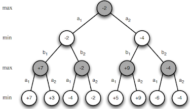
- 그림에서 leaf node가 end-game state라고 치자. 두 player가 minimax policy로 플레이 하고 black이 먼저 수를 둔다면, 마지막 state의 직전 state에서 black은 무조건 자신이 얻을 value가 높아지는 걸 택할 것이다 (즉, 왼쪽부터 순서대로 \(v_{*}=7,-2,9,-4\). 그 이전 state에서는 white가 무조건 자신의 얻을 value가 높아지는 걸 택할 것이다 (best response). Zero-sum game이므로 이는 black이 얻을 value가 낮아지는 쪽을 택하는 것과 같다 (minimax). 이런 절차로 black의 현재 state에서의 (minimax) value를 구하면:

- 즉, 승부는 이미 black의 패배로 결정났다.
Drawbacks of Minimax Search
- Search tree grows exponentially
- Impractical to search to the end of the game
- Instead, use (minimax) value function approximator \(v(s, w) \approx v_{*}(s)\)
- E.g., binary feature vector (장기말의 생존 유무 등) with linear weighting
- Note: 아직 learning은 아니기 때문에 이 weight는 search 과정에서 학습하는 게 아니라 고정. Hand-crafted value function (no learning).

- Minimax search run to a fixed depth
- Use value function to estimate minimax value at the depth
- Example: Deep Blue
- 8000 handcrafted chess features
- Binary-linear value function
- Weights are largely hand-tuned by human experts.
- 현실에서는 Alpha-beta pruning 등을 이용하여 tree의 branch 중 굳이 탐색할 필요없는 branch를 삭제하는 식으로 search space를 더욱 줄인다.
Learning with Minimax Search
- Why don't we learn the value function approximator?
- 위 value function approximator의 성능을 게임이 진행함에 따라 발전시키는 게 자연스러운 아이디어 확장이다.
- \(\Rightarrow\) self-play RL
Self-Play Reinforcement Learning
- Classic game은 rule이 이미 정해져 있다. 따라서 일종의 known MDP이다. 따라서 model-based RL에서 simulation-based planning을 하여 data augmentation 효과를 내는 것처럼 실제로 (예를 들면) 체스 대국 도중에 스스로 self-play해서 전략을 도출할 수 있다.
- 1. 일단 value function approximator을 학습한다. (learning)
- 2. 그 후 minimax search with VFA를 통해, 일정 depth(시간) 미래의 state의 (approximated) minimax value를 근거로 action을 선택한다. (searching)
- Note: Sarsa revisited

- Define \(v(s, w) \approx v_{*}(s)\)
- Policy improvement
- For deterministic games, \(q(s,a) = v(s')\) since \(s'\) is deterministic given \(s, a\). Let's define such mapping as \(s' =succ(s,a)\).
- \(\pi^1(s) = \underset{a}{\mathrm{argmax}} \; v(s'=succ(s,a), w)\)
- \(\pi^2(s) = \underset{a}{\mathrm{argmin}} \; v(s'=succ(s,a), w)\)
- Greedy for each player
- Value function or value approximator update: MC, TD(0), TD(\(\lambda\)), etc.

- 하던대로 하면 됨
- Minimax search with VFA
- Minimax search run to a fixed depth
- Use the value function approximator to estimate minimax value at the depth
Combining Reinforcement Learning and Minimax Search
- Monte Carlo Tree Search같은 simulation-based search를 model-based RL에서 이용했던 것처럼, minimax search를 RL에 이용하여 좀 더 의미있고 똑똑한 방식으로 value를 추정해보자.
- 다만 minimax search는 정말로 가능한 branch를 (특정 depth까지) 다 탐방해보고, simulation-based search는 sampling을 통해 일부 branch만 탐방한다는 차이점이 있다.
- 위의 TD(0) 알고리즘은 value approximator 학습 초기에는 \(v(S_{t+1}, w)\)가 굉장히 의미없는 값일 가능성이 높다. Minimax policy가 Nash equilibrium인 걸 알기 때문에 search를 통해 좀 더 전략적으로 value function approximator를 update할 필요가 있다.
- 가정: deterministic game
- TD root
- Define: \(l_{+}(s)\) is the leaf node achieving minimax value from \(s\).
- Minimax search with VFA의 경우처럼, \(s\)에서 minimax policy로 tree search를 진행할 때 tree의 최대 깊이 앞(미래)에 있는 node
- (exhaustive search 불가능하므로 미리 tree의 최대 깊이를 특정해둠)
- Take initial action: minimax policy와 \(v(S_{t+1}, w)\)에 따라 \(S_{t+1}=s_{t+1}\)을 실제로 택한다 (또는 \(\epsilon\)-greedy 등 적절히 exploration을 위한 randomness를 추가하여).
- Value function backed up from search value (kind of simulation) at next state:
- \(v(S_t,w) \leftarrow v(l_{+}(S_{t+1}),w)\)
- Search tree depth를 2로 설정한 TD root algorithm 예:

- Note: 왜 \(S_{t+1}\)의 value는 무시하고 그보다 더 미래의 state의 approximated value로 backup을 하는지 궁금할 수 있는데, 실제로 minimax policy를 적용해서 미래 state \(l_{+}(S_{t+1})\)를 찾은 것이므로, 이상적으론 \(l_{+}(S_{t+1})\)의 true minimax value나 \(S_{t+1}\)의 true minimax value나 실은 같은 것이어야 한다 (아래 minimax search 예시 그림 참고). TD root는 \(v_{*}(S_{t+1})\)를 더 잘 근사하는 게 \(v(S_{t+1},w)\)보단 \(v(l_{+}(S_{t+1}),w)\)라고 가정하는 것이다.
- TD leaf
- TD root에서는 \(v_{*}(S_{t+1})\)를 더 잘 근사하는 게 \(v(S_{t+1},w)\)보단 \(v(l_{+}(S_{t+1}),w)\)라고 가정했다. TD leaf는 한 발 더 나아가, \(v_{*}(S_{t})\)를 더 잘 근사하는 게 \(v(S_{t},w)\)보단 \(v(l_{+}(S_{t}),w)\)니까 \(v(l_{+}(S_{t}),w)\)를 업데이트하자 제안한다.
- \(v((l_{+}(S_t),w) \leftarrow v(l_{+}(S_{t+1}),w)\)

- TreeStrap
- TD root와 TD leaf에서는 minimax policy와 \(v(S_{t+1}, w)\)에 따라 \(S_{t+1}=s_{t+1}\)을 일단 택하고 (real play) update를 어떻게 할지 고민했다 (search).
- TreeStrap은 search에 집중한다.
- 또한, TD root와 TD leaf는 minimax search 이후 오직 하나의 node만 update했다.
- TreeStrap은 minimax search로 방문한 모든 노드를 업데이트한다.
- 현재 노드 \(S_t\)와 그의 모든 자식 노드 \(s\)에 대해 (특정 depth까지, leaf node를 제외한),
- \(v(s,w) \leftarrow v(l_{+}(s),w)\)
- TreeStrap에서 현재 노드를 root로 (특정 depth까지) minimax search를 한 뒤 search tree의 모든 노드의 value를 업데이트하는 모습:

- Note: TD leaf는 현재 state에서도 self-play를 통해 \(v_{*}(S_{t})\)를 추정해야 하고, action sampling을 해서 얻어진 다음 state에서도 self-play를 해서 \(v_{*}(S_{t+1})\)를 추정해야 한다. 그 후 이 두 값을 가중치 합해야 한다. 이는 두 가지 self-play (uncertainty)를 동시에 취하는 거라 불안하다. 또 게임 초반에는 value approximator가 상당히 부정확하므로 action sampling해서 다음 state의 정보로 backup하는 게 불안할 수 있다. TreeStrap은 그런 문제 의식에서 출발했다.
Monte-Carlo Search and MC Tree Search in Games
- Good material: Minimax and Monte Carlo Tree Search - Philipp Muens

- UCT = MCTS의 \(\epsilon\)-greedy 알고리즘을 UCB algorithm로 교체 \(\rightarrow\) guarantee to explore all paths of the tree

Reinforcement Learning in Imperfect-Information Games
- Imperfect-information games: Blackjack


- 상대방의 action, state를 제대로 알 수 없는 imperfect game의 경우, UCT 단순한 MCTS를 쓰면 Nash equilibrium을 찾을 수 없다. 수렴하지 않는다. 따라서 모든 적의 average behaviour를 학습한 뒤 이에 대한 best response를 도출하여 gradient smoothing 같은 효과를 낸다 (매 update의 노이즈를 줄인다고 생각하자). 따라서 일반 UCT보다 강건하다.


댓글
댓글 쓰기